![]()
Introduction
Thank you for reading Part II of this three-part series on water management. In Part I we discussed the importance of having a written water management plan, the advantages of Regulated Deficit Irrigation (RDI), monitoring water quality and soil water-holding capacity, and vine water status as a measure of water stress. In this second part in the series, we focus on irrigation (Sections 5.6 to 5.11 of the Lodi Winegrower’s Workbook).
This Coffee Shop article is an expert from the Lodi Winegrower’s Workbook (Chapter 5: Water Management). The Workbook is a comprehensive, practical, and user-friendly guide to farming winegrapes. The Lodi Winegrape Commission has handed out hundreds of copies over the years, and growers continue to pick more up at our monthly educational meetings. Workbooks are free to all Crush District 11 (Lodi) growers, and can be ordered from the Commission: (209) 367-4727. Click HERE to learn more.
Irrigation scheduling for mature vines
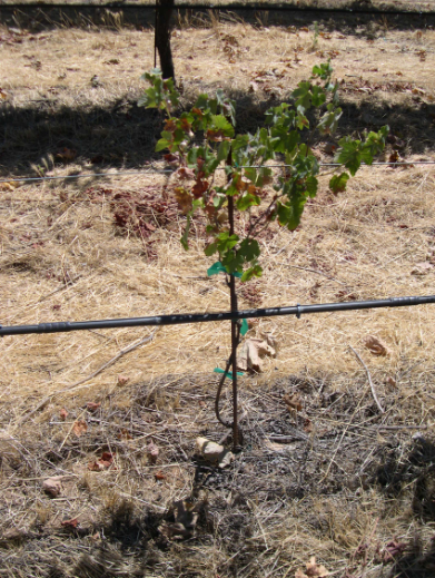
Water-stressed replanted vine
Irrigation of young replanted vines: Irrigation management should always take into consideration the age of the vines. For young vines like this replant, under-irrigating can be detrimental to growth and the vine may be slow to recover from it. The young replants in this vineyard did not receive enough irrigation resulting in basal leaf burn and stunted growth. The grower will struggle to get strong growth from these vines and, in turn, will struggle with training.
A simple solution is to irrigate the entire vineyard for one to two hours a day providing the young replanted vines with sufficient water for healthy growth, but not disrupting the irrigation scheduling program that the grower is employing in the rest of the vineyard.
Estimating full potential vineyard water use: Using a RDI % requires an estimate of full potential water use. The full potential water use varies as a result of climatic conditions and the size of the canopy. The climate factor can be estimated using the reference evapotranspiration (ETo) values, which indicate that vine water use varies over the season. Normal or average year’s ETo data (1984- 2003) is shown for Lodi, California in Figure 5.2. Water use is also influenced by vine canopy growth from bud break to full canopy expansion. Canopy growth is accounted for by a modifying factor of the ETo called the Crop Coefficient (Kc). The Kc varies from a small value after bud break and increases as the vine canopy expands to maximum size. Together, these factors (ETo × Kc) contribute to a water use pattern that begins at a low rate in spring, peaks in mid-summer, and then declines as leaf drop approaches. Canopy management practices such as hedging and leaf removal or canopy disruption by machine harvesting can further modify this pattern by reducing the solar energy interception by the vine and therefore the Kc. When considering the water use of a single vine, a larger canopy will have a larger leaf area exposed to the atmospheric conditions that drive water use and, therefore, that individual vine will have a greater water use.
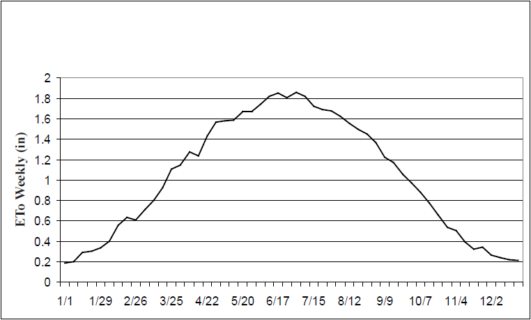
Figure 5.2. Average ETo’s throughout the year for Lodi from 1984 to 2003
When estimating the full water use of an area of land planted to winegrapes (ETc), it is necessary to quantify the extent of canopy coverage by measuring the percentage of land surface shaded by the vine canopy. Row spacing can have a significant influence on percent land surface shaded since a closer row spacing increases the land surface shaded by the vines. The amount of land surface shaded can also be affected by trellis design, vine health, and vigor as a result of rootstock/scion combination, soil conditions, pests that affect leaf area or root function, and fertilization. In addition, vine training, trellis type, and spring growth conditions can influence the rate of canopy expansion thus emphasizing the fact that the percentage of land surface shaded increases as the canopy develops. The variables that affect land surface shading will subsequently affect vine water use.
__________________________________________________________________________________
Vine water use increases as the percent of land surface shaded increases. The practical ramifications are that wider spaced rows, young grapevines or low vigor vines with a small canopy have a lesser percentage land surface shaded and use less water on a per-acre basis than vines with a larger canopy.
__________________________________________________________________________________
The percentage of land surface shaded is measured midday (solar noon). The method described in the next section for estimating land surface shading seems to work well with bilateral or quadrilateral trellis systems, but less well in vertical shoot positioned (VSP) vineyards. VSP canopies have the minimum land surface shaded at solar noon when row orientation is north/south and therefore may require a different method to account for the canopy/land surface relationship. Research is currently underway to develop a reliable method for use with VSP and similar trellis systems.
Evapotranspiration reference values (ETo): Evapotranspiration Reference Values (ETo) are calculated using measurements of climatic variables including solar radiation, humidity, temperature, and wind speed and expressed in inches or millimeters of water. A one-inch depth of water use, like rainfall or irrigation water, is equal to 27,158 gallons per acre of land. ETo values most closely approximate the water use of a short mowed full coverage grass crop. Climatic conditions are constantly collected from which ETo values are calculated and made available by CIMIS. The California Irrigation Management Information System (CIMIS) is managed by the State of California Department of Water Resources, which collects, maintains and provides Reference Evapotranspiration (ETo) values from nearly 100 weather stations throughout California. Both historical averages (normal) and real time (current year) values are available. CIMIS is on the web at: http://www.cimis.water.ca.gov.
Crop coefficient (Kc): The Crop Coefficient (Kc) is a factor, which allows the use of Reference values (ETo) to estimate full grapevine water use (ETc) of a non-water stressed vineyard. Kc values have been experimentally linked to the percent shaded area in the vineyard measured at midday. They can be measured at any time of the season, however when using the Stress Threshold Method, it is necessary to only measure at the threshold or beginning of irrigation. At that time, canopy expansion is complete. It should be re-measured if canopy reductions occur due to canopy management such as hedging.
Larry Williams, professor of Viticulture at UC Davis, demonstrated in a weighing lysimeter at the University of California Kearney Research and Extension Center that vineyard water use and Kc increases linearly with the percentage of land surface shaded by the crop. He suggests measuring the percent shaded at midday and using the following equation to determine the Kc:
Kc = 0.002 + 17 x the percent shaded area
Simplified Equation: Kc = 1.7 x percent shaded area (e.g., 0.40 for 40%)
The procedure would entail measuring the average shade on the floor at midday. For example, let’s look at the vineyard illustrated in Figure 5.2 below with an 11 foot row spacing and a 7 foot vine spacing. The average amount of shade between two vines is measured at 31 sq ft then compared to the single vine area of 77 sq ft which is 40% of the square foot area of one vine. The Kc is calculated as follows:
Kc = (1.7 x 0.40) = 0.68
[need original photo for Fig 5.2]
Calculating full potential water use with historical average ETo. The best way to illustrate the mechanics of calculating the amount of water to apply is to select a vineyard with specific site and other conditions and perform the calculations using a spreadsheet. The specific vineyard conditions in the above example are as follows:
Variety: Cabernet Sauvignon, mature
Spacing: 7 x 11 feet bi-lateral cordon
Leaf water potential Stress Threshold: -13 bars reached July 8th
Shaded area: 40% or 0.40
Kc = 0.68
Area: Lodi, CA CIMIS stations #42 and # 166
Harvest: October 1st
The spreadsheet will be divided into 3 parts to illustrate each step. The first step is to calculate full potential water use of the vineyard.
Table 5.3 shows an example calculation of weekly full potential water use for Lodi, California using the 1984 to 2003 historical average ETo for CIMIS stations #42 and #166. After the -13 bar threshold was achieved (July 8 in this example), the net irrigation requirement can be calculated in weekly increments from the threshold date to the end of the season using average historical ETo values. The Kc used is 0.68 for a 40% midday shaded area. Calculations are made only after the threshold midday leaf water potential (-13 bars) was measured in the vineyard on July 8. The product of ETo and Kc yields the full potential water use: ETo × Kc = full potential water use (ETc).
__________________________________________________________________________________
Table 5.3.: Irrigation scheduling worksheet – Lodi, CA
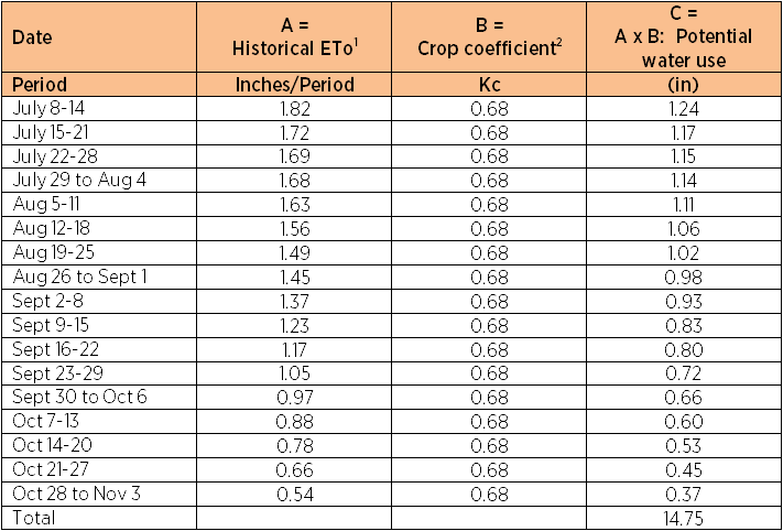
(1) http://www.cimis.water.ca.gov/cimis or http://ucipm.ucdavis.edu.
(2) Crop Coefficient calculated based on 40% midday land surface shaded (0.68)
ETo are the averages of daily data from 1984 to 2003 from the Lodi #42 and West Lodi #166 weather stations.
Assumptions:
1. Leaf water potential stress threshold was reached July 8th.
2. Harvest date was October 1.
__________________________________________________________________________________
Calculating the water use using the regulated deficit % (RDI%): Once the full potential water requirement is calculated for the vineyard, the Regulated Deficit percent (RDI%) is used to calculate the amount of water the vineyard will use under the RDI% you have selected. In our example, 0.50 or 50% of full potential water use was selected. Table 5.4 shows the full potential water use x RDI% equals the net amount of water use for the selected RDI%. Notice the RDI% increased to 1.0 or 100% after harvest as full water is required to encourage root growth, nutrient uptake and further carbohydrate accumulation. An increase in RDI% to near 100% is common with extended maturity harvests near 19º Brix measured by berry sampling.
__________________________________________________________________________________
Table 5.4. Irrigation scheduling worksheet – Lodi, CA
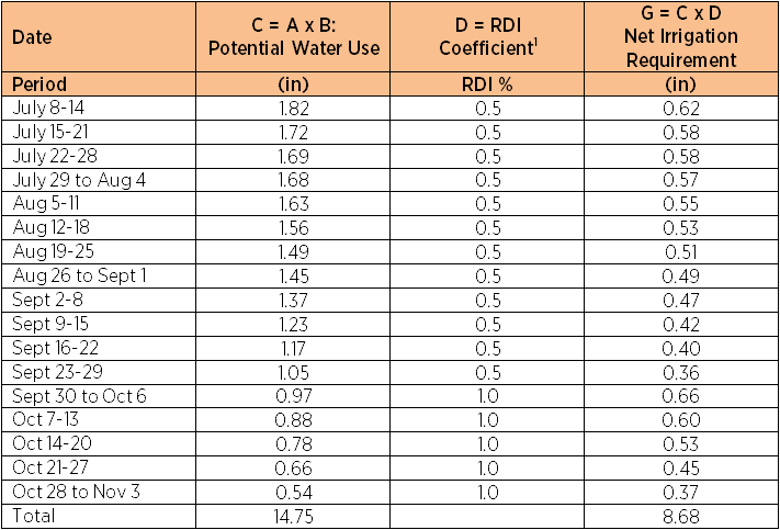
(1) Regulated Deficit is 50% (0.50)
ETo are the averages of daily data from 1984 to 2003 from the Lodi #42 and West Lodi #166 weather stations.
Assumptions:
1. Leaf water potential stress threshold was reached July 8th.
2. Harvest date was October 1.
__________________________________________________________________________________
Adjusting the schedule for the current season’s climate: Weekly historical ETo values were used in the above spreadsheets. As real time (the current season) ETo and effective rainfall values become available, they can be substituted into the table for the historical averages to account for the variance from normal ETo values. Real time ETo and rainfall are available on a one day lag time from the CIMIS network.
This method of irrigation scheduling relies on a calculation using historical ETo data for a one-week period, calculating the RDI water requirement then applying the indicated amount of water to the vineyard. After the end of that week, the real time data is downloaded and substituted into the spreadsheet to replace the historical ETo used to develop the last week’s schedule. Any differences between the previous week’s application volume/time should be adjusted as an addition or subtraction on the new, current week’s schedule. For example if 12 hours were applied using the historical ETo values then upon re-calculating using real-time data the amount should have been 11 hours, simply subtract 1 hour from the current week’s schedule.
In order to react to rapidly changing climate, if an extraordinary hot and low humidity period begins and is expected to last a few days—increase the irrigation volume to try to meet the increase in water use. When recalculating with real time ETo values, the next week’s result will indicate your success in estimating the increased water use.
Accounting for the soil water contribution and effective rainfall: Adding both soil water extraction and effective rainfall to the spreadsheet can further improve the estimated volume of irrigation water necessary to optimize the irrigation strategy.
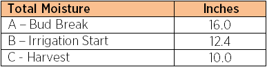
The soil moisture content declines as the vine extracts moisture from the beginning of shoot growth until the leaf water potential Stress Threshold is reached. At this time, the vine can still remove additional moisture from the root zone until harvest; the available moisture is at deeper depths, and the rate of extraction is slow. This water must be accounted for as an input to vine water use in column E Table 5.6. In deep (7 ft) medium texture soils, an average amount of water which will be removed from the irrigation start to harvest is typically 2½ inches. On shallower soils, this amount can be as low as 1 inch. Using a calibrated soil moisture-measuring instrument which reads in inches of total water per foot of soil, the water content of the root zone can be measured at bud break, the Stress Threshold and at harvest. These times represent the root zone starting point, the irrigation start, and the dry point respectively. Subtracting the irrigation start moisture content form the bud break content will represent the amount of soil moisture used until the start of irrigation. Additionally, subtracting the harvest (dry point) from the volume at the irrigation start represents the volume of water the vines will use from that point through harvest.
Table 5.5 shows the readings typical of a 7 ft depth sandy loam soil in Lodi, California. If soil measurements are not available, use the estimations described above.
__________________________________________________________________________________
Table 5.5. Total root zone soil moisture content
 __________________________________________________________________________________
The water that will be used from the Stress Threshold to harvest is called the soil contribution in Table 5.6. Divide the amount (in this example, 2.5 inches) by the weekly periods from the Stress Threshold to the estimated harvest date, July 8 through Sept 30.
2.5 inches / 12 weekly periods = 0.2 inches per period
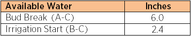
Table 5.6 illustrates the addition of the estimated soil contribution of each weekly period from the threshold to harvest (Column E).
Effective rainfall is usually minimal in the period of time from the Stress Threshold through harvest. However, significant rainfall is possible and must be accounted for as a water source to meet the calculated vine requirement. Effective rainfall is not considered unless it is greater than three times the daily ETo. The most practical method to estimate effective in-season rainfall for vineyards is using the formula:
Effective Rainfall = [If rainfall exceeds 3 ETo (in) – 0.25 in] × 0.8
This method discounts the first 0.25-inch as lost to evaporation after the event and estimates 80% of the remainder is stored in the soil for vine use. In Table 5.6, the effective rainfall (column F) is entered into the week beginning October 28. The measured rainfall was 0.65 inches. Three times the daily ETo – 0.23 in. Calculations are as follows:
Effective Rainfall = [0.65 -0.25] × 0.8 = 0.32 in.
Notice that the 0.32 inches is nearly equal to that week’s calculated vine use and the irrigation volume is reduced to near zero for that week period.
__________________________________________________________________________________
Table 5.6. Irrigation scheduling worksheet – Lodi, CA
(1) Regulated Deficit is 50% (0.50)
(2) Effective rainfall is calculated from actual rainfall (calculations are shown above)
ETo are the averages of daily data from 1984 to 2003 from the Lodi #42 and West Lodi #166 weather stations.
Assumptions:
1. Leaf water potential stress threshold was reached July 8th.
2. Harvest date was October 1.
__________________________________________________________________________________
Energy issues related to irrigation pumping
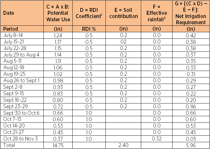
Solar array that produces the electricity for the pump in the foreground
Farming the sun: Winegrowers already farm the sun with the solar energy collectors found in grape leaves; why not farm the sun for electrical energy?
Photovoltaic solar panels capture the light energy of the sun and convert it to
direct current power. When connected to the electric utilities power grid and time-of-use metering, a solar system can capture energy during the daylight hours sending the power to the grid at the peak hourly rate and retrieving energy from the grid, to run an irrigation pump, during the night at the off-peak rate.
So, a solar system is effectively delivering power to the grid for a higher price than
an irrigation pump running at night is drawing out of the grid. This advantage helps recoup some of the costs of installing the system. However, it should be noted that in the current system, total credit cannot exceed actual use for the day or season.
A net metering time-of-use system keeps track of the power produced by the solar panel and banks that power for when the energy is later drawn. Another advantage of a system like this is that power is produced year round, so all the energy captured on the 300+ sunny days a year in Lodi can be drawn when needed at no cost.
Unfortunately, because a grid connected system is just that, connected to the grid, when a power outage occurs, energy is not delivered. Alternatively, an off-the-grid system has the advantage of being able to supply power during a power outage from a large number of batteries, but the cost is significantly higher. For relatively small systems like those used to run an irrigation pump, a time-of-use grid-connected system has the most advantages.
Pump efficiency tests make economic sense: Field testing programs have shown that overall efficiencies for electrically driven pumps average less than 50 percent, as compared to a realistically achievable efficiency of at least 67 percent. This implies that 25 percent of the electrical energy used for pumping is wasted resulting from poor pumping efficiencies alone. Depending on acreage and water volume pumped, winegrowers could significantly reduce energy costs per well by increasing pumping plant efficiencies from present average levels to higher levels.
__________________________________________________________________________________
Common causes for poor pumping plant performance:
- Wear (sand)
- Improperly matched pump
- Changed irrigation conditions (Irrigation system changes; Ground water levels)
- Clogged impeller
- Poor suction conditions
- Throttling the pump
__________________________________________________________________________________
Many public utility companies will cost share the price of a pump test. For more information, contact the Agriculture Pumping Efficiency Program, The Center for Irrigation Technology, CSU, Fresno www.pumpefficiency.org.
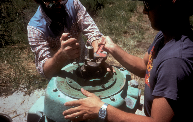
Bowl adjustment on turbine pump to improve pumping efficiency
__________________________________________________________________________________
Table 5.3. Irrigation scheduling worksheet – Lodi, CA
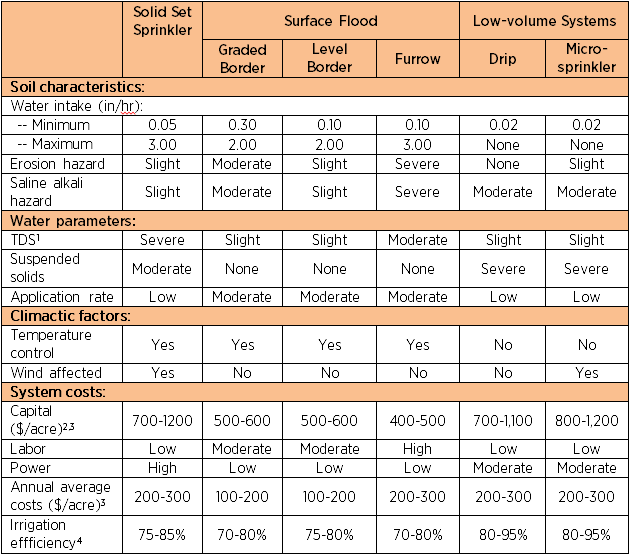
(1) Total dissolved solids
(2) Amortized capital costs plus operation and maintenance costs
(3) While the costs will become dated, they do indicate the relative differences in costs among the various types of irrigation systems.
(4) Irrigation efficiency = consumptive use + applied water; assuming good to excellent management and design
__________________________________________________________________________________
Distribution uniformity of above ground low volume irrigation systems
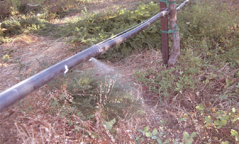
The distribution uniformity of this irrigation system is in desperate need of maintenance
Determining the average application rate and distribution uniformity of low-volume irrigation systems (Prichard et al. 2004):
- Drip emitter discharge may vary with the pressure, manufacturing variation and clogging in the drip system. For example, a 0.5 gallons per hour (gph) dripper may not actually be discharging at 0.5 gph.
- If there are multiple irrigation blocks, each block should be evaluated separately since they may be operating at different pressures.
- Sample drip emitters at the following locations:
- Head of the system:
- 4 near the head of the lateral
- 4 near the middle of the lateral
- 4 near the end of the lateral
- Middle of the system:
- 4 near the head of the lateral
- 4 near the middle of the lateral
- 4 near the end of the lateral
- Tail end of the system:
- 4 near the head of the lateral
- 4 near the middle of the lateral
- 4 near the end of the lateral
- Head of the system:
In addition, you might sample at any other spots where you suspect there could be a difference in the pressure and discharge rate. For example, low or high elevation spots in the vineyard.
More emitters than suggested above should be sampled on large irrigation blocks (greater than 20 acres).
- Collect water for 30 seconds in a 100 ml graduated cylinder (see Table 5.8) or in a 35 mm film canister (see Table 5.9). Use either table to convert the amount of water collected from each sampled emitter to the discharge rate for that emitter.
A. Determine the average application rate:
For each irrigation block, average all your discharge rate measurements. This is the average emitter discharge rate (gph) of your emitters.
Example: If you measured the output from 36 drip emitters, find the average discharge rate (gph) of the 36
emitters:
- Assume the average discharge rate was calculated at 0.48 gph.
- Assume there are 2 emitters per vine.
Average Application rate per vine (gph) = 0.48 gph per dripper x 2 drippers per vine = 0.96 gph/vine
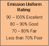
B. Determine the emission uniformity:
Each drip emitter in the vineyard will be discharging water at a different rate. This discharge variability is due to manufacturing variation between emitters, pressure differences in the system, and any emitter clogging which may be occurring.
The drip system’s application uniformity is quantified using a measurement called the Emission Uniformity (sometimes referred to as the Distribution Uniformity). The Emission Uniformity (EU) is defined as:
![]()
To determine the average discharge rate of the lower 25% of sampled emitters, the discharge
rate (gph) of each of the sampled emitters should be ranked from lowest to highest and the 25%
of the emitters with the lowest discharge rate should be averaged together. For example, if 36
emitters were monitored, the average of the 9 emitters with the lowest discharge rates would be
determined.
Example continued:
- Average discharge rate of all sampled emitters = 0.48 gph
- Average discharge rate of the low 25% sampled emitters = 0.48 gph
![]()
Poor emission uniformity (<70%) requires a close look at the systems pressure differences sometime due to pressure regulator adjustment or filter clogging. Emitter clogging is not uniform, usually occurring to a greater extent in emitters towards the end of the poly lines. Remedial actions should be taken considering the type of clogging that occurs.
__________________________________________________________________________________
Table 5.8. Drip emitter discharge rate (gallons per hour or gph) using a graduated container (100 ml graduated cylinders work well)
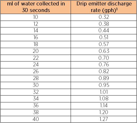
(1) Drip emitter discharge rate (gph) = water collected (ml) x 0.0317 (seconds)
__________________________________________________________________________________
Table 5.9. Drip emitter discharge rate (gallons per hour or gph) using a 35mm film canister
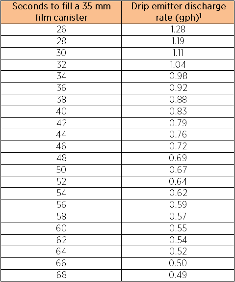
(1) Drip emitter discharge rate (gph) = 33.29 / time to fill 35 mm film canister
__________________________________________________________________________________
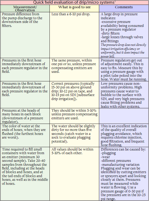
(1) Charles M. Burt, Cal Poly Irrigation Training and Research Center (ITRC)
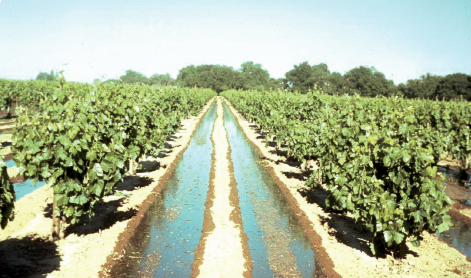
Figure 5.3 Furrow irrigation showing uniform wetting
Measuring distribution of infiltrated water under surface flood or furrow systems is difficult at best. However, the overall goal is to provide near equal opportunity time along the length of the furrow or check. Figure 5.3 shows a relatively flat vineyard using large furrows which are filled quickly providing reasonable distribution.
